
What a million tokens costs on-prem: H100 vs H200 vs API
What a million tokens costs on-prem: H100 vs H200 vs API
Reading time: about 9 minutes. Cluster: architecture. Author: Fryderyk.
The answer first
The cost of a million tokens on your own GPU does not come from the price of the card or the peak throughput in a benchmark. It comes from one division: the hourly rate of the card divided by the number of tokens the card will actually produce in that hour. And that number depends on utilization, not on what the card can squeeze out at full saturation.
At full saturation, a node built on H100-class cards serves an open-weight model in the 70B class for roughly 0.55 USD per million tokens, while the newer H200, thanks to higher memory bandwidth, drops closer to 0.35 USD. Both figures sit near what a managed API charges for the same class of model, about 0.60 USD per million tokens. The catch is that 0.55 and 0.35 only hold when the card works without pause. At 25 percent utilization the effective cost rises fourfold, because you pay the same for idle hours. The API has no such problem, because you pay only for tokens that actually came out.
The conclusion: your own GPU beats the API on pure compute cost only above very high, steady utilization. The H200 pushes that threshold clearly downward against the H100, but it does not erase it. Below the threshold, the argument for on-prem is data control and compliance, not cost per token. Below, I take that division apart step by step.
Table of contents
- Why peak throughput is the wrong number
- The formula: from hourly rate to cost per million tokens
- H100 vs H200: what really separates these cards on 70B inference
- Table: cost per million tokens at full saturation
- The variable that flips the math: utilization
- Table: effective cost by utilization
- The break-even against the API
- Why the naive calculation falls apart
- How this differs from the TCO calculator
- FAQ
- Disclosure and biases
- What I do not cover here
- Related notes
Why peak throughput is the wrong number
A card in an inference-server benchmark reports peak throughput: how many tokens per second it squeezes out at full batch, maximum concurrency and ideal load. That number is useful for sizing and for comparing hardware against hardware, and I wrote about it separately for Llama 3.1 70B. For a cost calculation it is misleading, because in production the card is almost never saturated.
A cost calculation has three floors, and most calculations stop on the first. The first floor is the hourly rate of the card. The second is how many tokens the card produces in an hour when fully loaded, that is throughput times 3600 seconds. The third, the one most often skipped, is what percentage of those hours the card was actually computing anything. Only after passing through all three floors do you get the number you can show a CFO: the effective cost per million tokens actually produced. Peak throughput describes only the second floor, and even that under an assumption production does not meet.
The formula: from hourly rate to cost per million tokens
The whole text rests on one formula, so it is worth writing out.
Cost per 1M tokens (at saturation) = node hourly rate / (throughput in tok/s x 3600 / 1,000,000)

Effective cost per 1M tokens = cost at saturation / utilization
The node hourly rate is not the rate for one card, but for as many cards as the model actually needs. A 70B-class model in BF16 does not fit on a single 80 GB card, so an H100 node is two cards. That is the first trap: comparing the price of one card with the price of the API when running the model takes two.
Throughput in this formula is the aggregate output of the server at high batch, not the speed of a single request. A server handling many requests at once produces far more tokens per second in total than any single user sees, and it is that aggregate number that divides the cost.
Utilization is the share of hours in which the node was actually computing, out of all the hours you pay for. A node exposed around the clock but queried only during one plant's working hours has utilization in the low double digits, even if it is saturated at peak.
H100 vs H200: what really separates these cards on 70B inference
Large-model inference, in the token-generation phase, is bound by memory bandwidth, not compute. So for cost per token what matters most is memory bandwidth, and here the H200 has a structural advantage.
The H100 is 80 GB of HBM3 memory and about 3.35 TB/s of bandwidth. The H200 is 141 GB of HBM3e and about 4.8 TB/s, roughly 43 percent more. More memory means a 70B-class model fits on a single H200 card with room to spare for context, instead of requiring two H100 cards. Wider bandwidth means the same model layer is read from memory faster, so the card generates tokens faster. In practice, on models of this class, that translates into throughput higher by about half, and in some TensorRT-LLM configurations more.
The cost consequence is not obvious. The H200 has a higher hourly rate than the H100, so at first glance it is more expensive. But because it produces more tokens in the same hour and more often fits the model on one card instead of two, the cost per million tokens comes out lower. A card that is pricier per hour can be cheaper per token. That is the heart of the comparison, and it is the number that counts if the model is meant to run under steady load.
Table: cost per million tokens at full saturation
All figures are indicative, based on public GPU rental rates from 2026 and on aggregate throughput for an open-weight model in the 70B class. They exist to show the method, not to serve as a price list. For your own decision, plug in your own rates and your own benchmark.
| Configuration (70B model) | Memory / bandwidth | Node rate | Throughput (saturation) | Cost / 1M tokens |
|---|---|---|---|---|
| Node 2x H100 80 GB (BF16) | 2x 80 GB / 3.35 TB/s | approx. 5.00 USD/h | approx. 2,500 tok/s | approx. 0.55 USD |
| Node 2x H200 141 GB (BF16) | 2x 141 GB / 4.8 TB/s | approx. 7.40 USD/h | approx. 4,000 tok/s | approx. 0.51 USD |
| 1x H200 141 GB (FP8) | 141 GB / 4.8 TB/s | approx. 3.70 USD/h | approx. 3,000 tok/s | approx. 0.34 USD |
| Managed API (70B class) | not applicable | pay per token | not applicable | approx. 0.60 USD |
Two things from this table. First, at full saturation your own GPU is in the same price league as the API, and a single H200 with FP8 quantization drops clearly below it. Second, this entire table assumes 100 percent utilization, so it describes the ceiling of what is possible, not the real bill. The real bill is what the next section does.
The variable that flips the math: utilization
The hourly rate of a card is fixed regardless of whether anyone is asking. A managed API works the other way: no requests, no bill. That is the whole difference between the two models, and it is what decides the outcome.
The effective cost per million tokens is the cost at saturation divided by utilization. A node that costs 0.55 USD per million at 100 percent costs 1.10 at 50 percent and 2.20 at 25 percent. Not because tokens get more expensive, but because a growing share of the bill pays for hours the node stood idle. The API's price per token stays flat through all of it.
That is why the question "H100, H200 or API" is badly posed until you know your utilization profile. A model exposed for an internal service desk, queried during one plant's working hours, has low utilization and loses to the API on pure cost, even if the card is saturated at peak. A model serving a steady, around-the-clock stream of requests from many sources has high utilization, and then your own GPU starts to make sense on cost too.
Table: effective cost by utilization
We take the 2x H100 node from the table above (0.55 USD per million at saturation) and the single H200 FP8 (0.34 USD at saturation) and divide by utilization. The API column is flat, because that is the nature of pay-per-token.
| Node utilization | 2x H100 (effective) | 1x H200 FP8 (effective) | Managed API |
|---|---|---|---|
| 100% | approx. 0.55 USD | approx. 0.34 USD | approx. 0.60 USD |
| 50% | approx. 1.10 USD | approx. 0.68 USD | approx. 0.60 USD |
| 25% | approx. 2.20 USD | approx. 1.36 USD | approx. 0.60 USD |
| 10% | approx. 5.50 USD | approx. 3.40 USD | approx. 0.60 USD |
The reading is brutal. The H100 node beats the API on pure compute cost only when it holds utilization above roughly 90 percent, which in practice means a steady, around-the-clock stream of requests. A single H200 with FP8 reaches parity with the API already at about 57 percent utilization, so the threshold is clearly easier to hold. That is a concrete, numeric argument for the newer card wherever load is moderate but not negligible.
The break-even against the API
The threshold can be computed directly. Your own GPU beats the API on compute when the cost at saturation divided by utilization falls below the API price. Rearranged: utilization has to be higher than the cost at saturation divided by the API price.
For the 2x H100 node: 0.55 / 0.60, about 92 percent utilization. For the single H200 FP8: 0.34 / 0.60, about 57 percent. The cheaper you are per token at saturation, the lower the utilization needed to beat the API, and that is why the H200 changes this calculation qualitatively, not just by a few percent.
Three levers move the threshold:
- Quantization. FP8 instead of BF16 roughly doubles throughput and lets the model fit on a single card, so it lowers the cost at saturation and with it the utilization threshold. It is the cheapest lever, because it needs no extra hardware, only acceptance of a minimal quality loss you have to measure on your own task.
- Model class. The whole calculation is about an open-weight model in the 70B class. A frontier model through the API costs many times more per token, which raises the reference price and drastically lowers the threshold at which your own GPU pays off. Conversely, a smaller 7 to 8B model is so cheap through the API that your own GPU will practically never win on compute alone.
- Availability mode. A node switched off outside working hours, if you rent and pay only for the hours it runs, artificially raises the utilization of the hours you count. That is the only way to bring your own GPU close to API economics at low traffic.
Why the naive calculation falls apart
Four mistakes that regularly produce a number you cannot defend in a board meeting.
First: dividing the card's rate by peak throughput and declaring that the cost per token. That skips utilization, the only variable that truly decides. The number comes out several times too low.
Second: counting one card where the model needs two. The 70B class in BF16 does not fit on 80 GB, so a real H100 node is two cards and two hourly rates. Count one and you understate the cost by half.
Third: using single-request throughput instead of the aggregate. A server at high batch produces many times more tokens per second in total than any one user sees. Costing by the speed of a single request overstates the cost and leads to the opposite, but equally wrong, conclusion.
Fourth: treating the H200 as more expensive because it has a higher hourly rate. Per hour, yes, but per token usually cheaper, because it produces more and more often fits the model on one card. A card pricier per hour can be cheaper per million tokens, and it is that second number that the decision is about.
How this differs from the TCO calculator
Here I count only the compute cost per million tokens, that is one line of the bill. That is a deliberate simplification, to show the mechanics of utilization without noise. A full TCO of an AI deployment also covers energy, people, compliance, project costs and exit, and compute there is usually the smallest and least differentiating line. I took that apart separately in the TCO calculator with a full worked example over three years.
The practical order is this: first compute the compute cost per token with this formula, to understand whether you are anywhere near the utilization threshold. If you are not, the discussion about your own GPU on a cost argument ends and moves onto the ground of data control. If you are, only then is it worth costing the full TCO, because compute stops being negligible and the rest of the lines start to decide.
FAQ
What does a million tokens cost on your own GPU?
At full saturation, a node with H100-class cards serves a 70B-class model for about 0.55 USD per million tokens, and a single H200 with FP8 quantization for about 0.34 USD. That is the ceiling. At real utilization below 100 percent the cost rises inversely: at 25 percent it is four times higher.
H100 or H200 for 70B-model inference?
Per hour the H200 is pricier, but per million tokens usually cheaper, because it has about 43 percent wider memory bandwidth, so it generates faster, and 141 GB, so it fits a 70B model on one card instead of two. If the model is meant to run under steady load, the H200 usually wins on cost per token.
When is your own GPU cheaper than the API?
On pure compute cost only above very high utilization: about 92 percent for a 2x H100 node and about 57 percent for a single H200 FP8, against an API price on the order of 0.60 USD per million tokens for the 70B class. Below those thresholds the API wins, and your own GPU is justified by data control, not price.
Why is the API sometimes cheaper despite expensive hardware on the provider's side?
Because you pay only for tokens that came out, not for the card's idle hours. An API operator averages utilization across many customers and keeps the cards near saturation, which a single company with one workload usually does not achieve. That is an advantage of the billing model, not pricing magic.
Does FP8 quantization ruin model quality?
Usually only slightly, but it has to be measured on your own task, not taken on faith. FP8 roughly doubles throughput and lets a 70B model fit on a single H200 card, so it is the cheapest lever for lowering cost per token, as long as the accuracy loss stays within your acceptance threshold.
// disclosure & biasesDisclosure and biases
I write from the perspective of someone working on an AI platform run outside the public cloud, so I have a natural inclination to stress the case for owning hardware. I tried to balance that with numbers that cut against the inclination: at moderate utilization, a managed API is cheaper on pure compute cost than your own GPU, and I show that plainly rather than hide it. The on-prem AI market has several categories of solutions, from self-assembly on open source, through productized platforms, to managed models, and each has a different cost profile. All figures are indicative, based on public GPU rental rates and API price lists from 2026, not on the outcome of any specific deployment. This is not financial or investment advice.
What I do not cover here
I do not compute the full TCO, that is energy, people, compliance and project costs, because that is a separate thread carried in the TCO calculator. I do not go into sizing for a specific model or the choice of quantization, because that depends on the task and deserves its own note. I do not compare specific API operators by name or quote their price lists, because they change every quarter; I give the method and the orders of magnitude. I do not discuss newer-generation cards or exotic multi-node configurations, because for a 70B-class model they do not change the conclusion about utilization. I also leave aside the cost and risk of maintaining your own hardware, which in a GPU-rental model look different from an owned server room.
Related notes
- GPU sizing for Llama 3.1 70B inference: numbers from benchmarks
- AI TCO calculator: methodology, a worked example and FAQ
- On-prem AI vs cloud TCO: how to calculate over three years
- AI architecture resilience: what you can audit on-prem
- Monitoring and observability for on-prem LLMs: what to log and how
Building CortexMine, an on-prem AI platform for European manufacturers under NIS2. Where this bias could affect conclusions, it is flagged inline.
Want to apply this to your case: architecture, compliance, and cost?
→ Book 30 min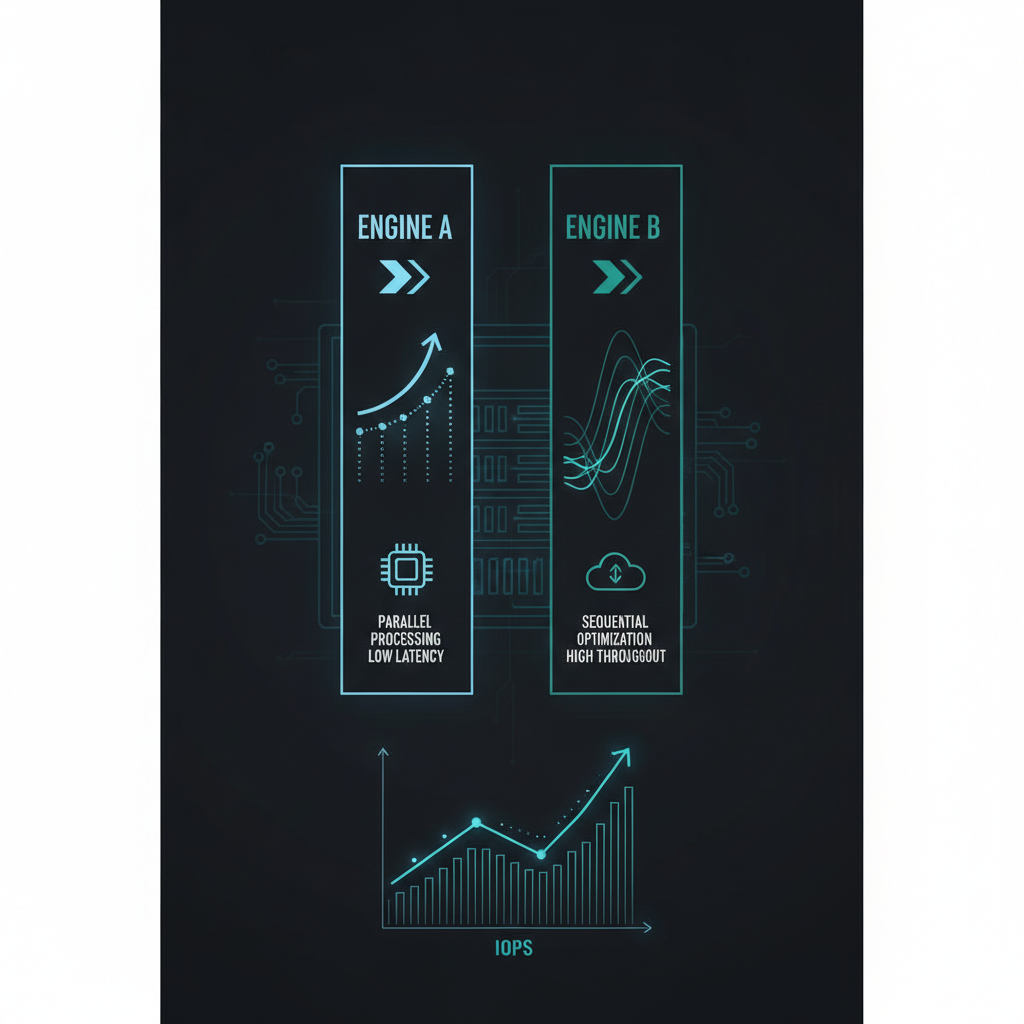
vLLM vs TensorRT-LLM: Which Engine for On-Prem LLM
GPU sizing tells you how many cards to buy. The serving engine decides how much you get out of them. vLLM vs TensorRT-LLM (and SGLang) on Llama 70B: throughput, TTFT, compilation cost and a decision table for on-prem.
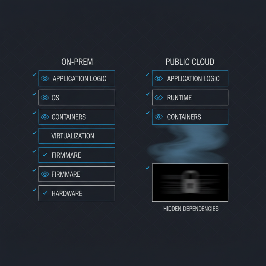
AI architecture resilience: what you can audit on-prem
The europe-west4 outage exposed something worse than downtime: you cannot audit the dependencies your AI runs on. What you can actually verify on-prem, and what a hyperscaler will never show you.
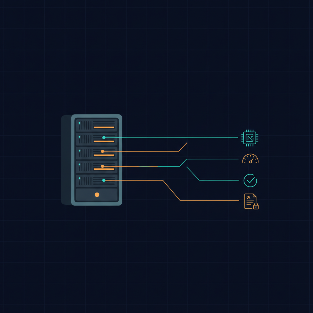
Monitoring and observability for on-prem LLMs: what to log and how
Four telemetry layers for an on-prem LLM: infrastructure, serving, quality and audit. What to log, what not to store, and how observability feeds the audit trail NIS2 expects.